XLOOKUP is usually used to search in one range to find a result in a a parallel range.
However, it can be used to find a result in an offset range.
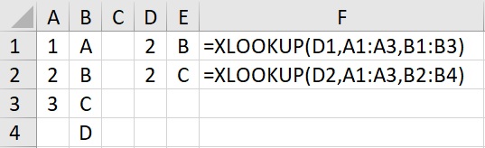
The first formula looks for 2 in the range A1:A3 and finds its result in the aligned rang e B1:B3 giving an answer of B.
The second formula uses an offset result range of B2:B4. 2 was the sedond element of the range A14:A3, so the formula finds the second element of the results range B2:B4. This gives an answer of C.
XLOOKUP is great at finding a result in a row or column based table, but what about if you need both. Say, the search items are in a column and the results are in a row. This can be achieved by using the TRANSPOSE function.
Using TRANSPOSE in the XLOOKUP function would look something like the following: =XLOOKUP(A1, “C1:C6”, TRANSPOSE(“D1:I6”))
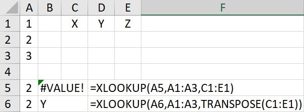
Using a column to find a result in a row produces and ‘#VALUE!’ error.
However, by wrapping the results range in the TRANSPOSE() function allows the formula to work normally.
The TRANSPOSE() formula works as an array formula. Array formulae also allow a mulitple lookup on a range such as a table.
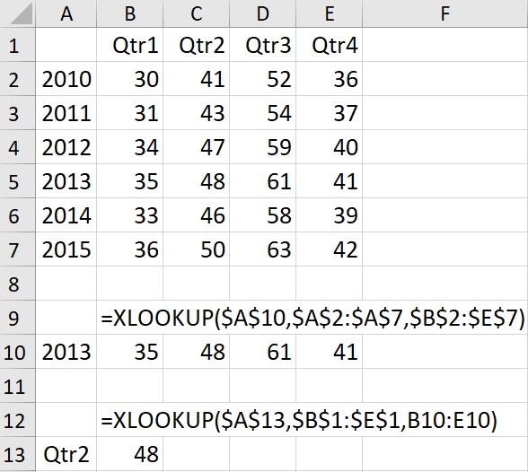
If you had a a table of a set of result by year and quarter, how would you find the result for a specific element?
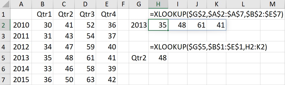
In the example below the formula in H2 is shown in H1. It searches in the 1 dimensional A2:A7 for a result in the 2 dimensional B2:E7. It thereby produces an array answer, showing the four quarterly results for the year in H2:K2.
The formula in H5 (shown in H4) then searches for ‘Qtr2’ in B1:E1 and having found it to be the second element, selects the second element of the array produced by the first formula.