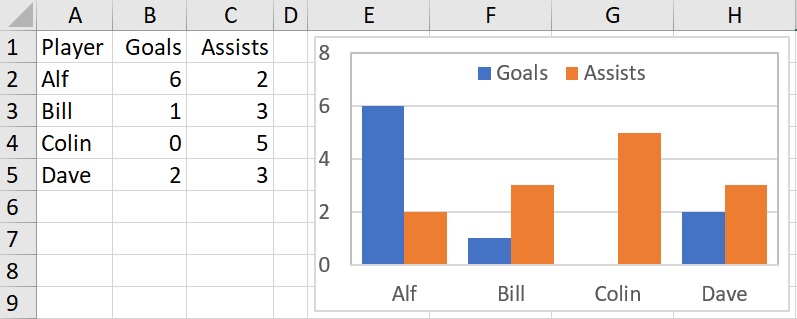
I have then created the chart series so that they are based on the range names (rather than formula). Note that range name must include the Workbook name. My workbook is ExcelTips.xlsx so the formula for the Goals series is: =SERIES(“Goals”,ExcelTips.xlsx!Player,ExcelTips.xlsx!Goals,1) The formula for the Assists series is: =SERIES(“Assists”,ExcelTips.xlsx!Player,ExcelTips.xlsx!Assists,2)
To make the chart dynamic we need to make these series dynamic. We need two functions for this:
COUNTA() This counts the number of non-blank cells in a range. (Note that the function COUNT() counts the number of cells containing numbers.) To count the number of players we need to find the number of entries in column A and subtract 1 for the title: COUNTA($A:$A)-1
OFFSET() Returns a reference to a range that is a given number of rows and columns away. The function works as follows:
=OFFSET(Reference, Rows, Cols, [Height], [Width])
Reference: Rows: Cols: Height: Width:
Reference from the offset is based Rows up or down to upper left cell Columns left or right to the upper left cell Number of rows of range [Optional] Number of columns of range [Optional]
Reference: Reference from the offset is based Rows: Rows up or down to upper left cell Cols: Columns left or right to the upper left cell Height: Number of rows of range [Optional] Width: Number of columns of range [Optional]
We are going to use the first cell of each of our series (Player, Goals and Assists) as our reference. This means that there is no need for an offset and the next two terms will be 0. Finally, we will use the COUNTA formula above to define the length of the range. (We don’t need the optional Width).
The three series are then:
=OFFSET(DynChrt!$A$2,0,0,COUNTA(DynChrt!$A:$A)-1)
=OFFSET(DynChrt!$B$2,0,0,COUNTA(DynChrt!$A:$A)-1)
=OFFSET(DynChrt!$C$2,0,0,COUNTA(DynChrt!$A:$A)-1)
Note that each of these formula are using the Player column to count entries so that the dimensions of the series will remain identical.
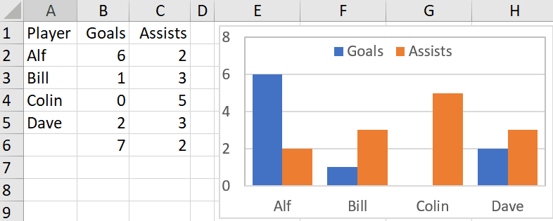
Now when an additonal player is added, the COUNTA function will increase by 1 and thereby so will the series.
In the example below I have already inserted the additional numbers to help demonstrate the change:
This mechanism is dependent on the first column being reserved for the player list. Your chart will have serious problems if you enter anything else in the column!
If your chart uses series in rows then the formula becomes =OFFSET(DynChrt2!$A$1, 0, 0, 1, COUNTA(DynChrt!$1:$1)-1) The 4th element now shows the height as 1 with the series length using the 5th element – Width.