Value to be found the Range to search for Value the Range to find the Result Result if SearchValue not found [Optional] Exact or Approximate value [Optional] Seach Ascending or Descending [Optional]
XLOOKUP operates in a way that is very similar to the LOOKUP function with the Optional Result Range used.
The Result Range does not need to be aligned with the Search Range, nor does it have to come after the Search Range. However, unlike with the LOOKUP function, the search and result ranges need to have the same orientation unless a further function is used.
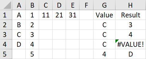
In the example below, there are 4 formulae in the range H2:H5:
The first searches A1:A4 and finds a result in B1:B4.
Next searches A1:A4 for an offset result in B2:B5.
Searching A1:A4 for a horizontal result in B1:E1 produces an error.
Finally, search B1:B4 for result in A1:A4.
Another important difference from LOOKUP() is that XLOOKUP() requires the Search and Results range to be the same size. Different size ranges will produce an error.
VLOOKUP() gave users the option of finding an approximate, smaller, variable by default or the exact match if selected.
XLOOKUP() gives the user these options:
0 – Exact Match – Default
-1 – Exact Match or next smaller
1 – Exact Match or next larger
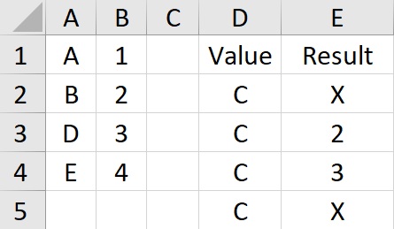
XLOOKUP() also adds the option for a result when exact match is not found.
The first searches looks for an exact match. As C is not found, the Not Found variable, “x”, is returned.
The next searches for the exact or next smaller. It finds B and returns 2.
Searching for the exact or next larger find D and returns 3.
Finally, searching with no match type marker defaults to an exact match search. As C is not found it returns “x”.
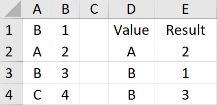
An important aspect of XLOOKUP() is that the order of the search entries does not matter, even when looking for an approximate result.
The last variable in XLOOKUP() changes the sort direction. The default is 1, which searches in ascending order. If the marker is set to -1 then the search is in descending order.
The Search Item. Range to be searched. Range of results. Answer if search term not found. Indicates wildcard search. Indicates reverse search.
“?arl” – The Search Item. $A$1:$A$4 – Range to be searched. $B$1:$B$4 – Range of results. “Not Found” – Answer if search term not found. 2 – Indicates wildcard search. -1 – Indicates reverse search.