VLOOKUP is apparently the third most used Excel function (after SUM and AVERAGE). I’m not sure how they know this.
It, and its horizontal sibling HLOOKUP, are very useful but care does need to be taken.
These two formula have more power than LOOKUP() because they can require an exact match. This in turn allows a search of a non-ordered range.
However, they are less flexible because the Search Range and the Result Range need to be in a single range. There is no direct ability for offsetting the lookup, for finding results left or above the search row or column, or for finding results in a range with different orientation.
The VLOOKUP function works as follows: =VLOOKUP(value, range, column, [approximate])
value: range: column: approximate:
value to be found the table of data to search the column number hodling the result approximate or exact [optional]
value: value to be found range: the table of data to search column: the column number hodling the result approximate: approximate or exact [optional]
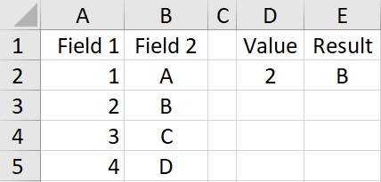
The formula in Cell E2 is:
=VLOOKUP(D2,$A$2:$B$5,2,FALSE)
The VLOOKUP function searches the left hand column of the range. In the example above, the formula looks for the value of D2, which is 2. It looks for this in the first column of the range, which is A2:A5. It finds the answer in cell A3. It then looks in the given column number for the result. The column number is 2 so the formula looks in the second column which is B2:B5. The final label is FALSE meaning it will not look for an approximate value. ie It will look for an exact match.
VLOOKUP(value,range,column,TRUE) and VLOOKUP(value,range,column) produce the same result.
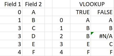
Searching for an approximate value can only be used when the seach column is in ascending order. Addtionally, the results can be unreliable if there are duplicates. With ascending order and no duplicates it will find the next lower value.
Looking up 0, 1 and 4 work as expected.
2 finds the next lowest value with marker set to True but produces error #N/A when set to False.
3 finds the result for the final entry for 3 with marker True and the first entry for 3 with marker set to False.
With the final marker set to False the function will look for an exact value. If the value is not found then the function will return an error #N/A.
However, with the final marker set to False, the search will work regardless of the order of search items. And, it will reliably find the first matching example where there are duplicates.
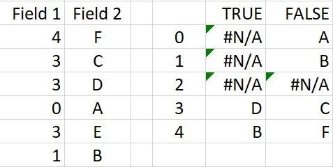
In the next example the search column is not ordered.
Setting the market to True produces very unexpected results.
However, with the marker set to True the formula finds the same results as for the ordered example (including finding the first row with 3 in Field 1).
A problem with VLOOKUP and HLOOKUP is when the table is edited.
Finding the result by column count rather than by column reference leads to problems.
If a column is inserted or deleted then the result will be taken from the wrong column.
Here Fields 2 & 3 are swapped.
VLOOKUP now returns a different answer.
(The formula LOOKUP continues to return the original answer. )
One final issue is that the range has to be continuous.
You can’t find the position in one range and the result for that position in another range or apply an offset to the result postion.