INDEX is a tool to target cells within an area. The function can be used to select individual cells, rows, columns or ranges within one or more given ranges.
The INDEX function works as follows: =INDEX(range(s), row, column, area number)
range(s): row: column: area number:
Usually a single range, but can be multiple ranges the row number within the area the column number the range number when there is more than one range
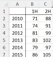
The formula to find the element in the 3rd row and 2nd column of the range is =Index(B2:C7, 3, 2) producing the answer 9
If the range has only one dimension then the second term works as row or column index: =Index(C2:C7, 3) = 99 =Index(B4:C4, 2) = 99
Excluding the third term when there are two dimensions causes an error: =Index(B2:C7, 3) = #REF!
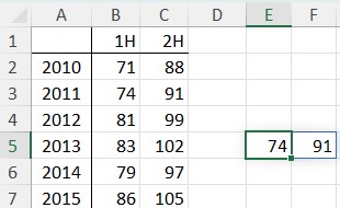
If a term is left blank (or as 0) then the row or column is selected as a dynamic array.
The formula in E5 is =Index(B2:C7, 2,)
There may be a case where the index is required accross multiple ranges. This can be achieved by separating the ranges with commas and wrapping the the set with parenthesis. The 4th term of the formula is required for selecting the addtional ranges.
The following formula finds the cell in the 2nd row and 2nd column of the 2nd range: =INDEX((B2:C4,B6:C7),2,2,2) = 105
One final method with INDEX is its use to create a range. The formula =Index(B2:C7, 3, 2) points to the cell C4. Therefore the formula =SUM(C2:INDEX(B2:C7,3,2)) finds the sum of the range C2:C4
MATCH or XMATCH can be used in conjunction with Index to retrieve cell contents.
MATCH requires the lookup range to be ordered, although it can be in descending order.
XMATCH does not require the series to be ordered
The MATCH and XMATCH functions are entered as follows: =MATCH(lookup value, array, match type)
lookup value: array: match type:
the value to be found the range to be searched find exact value, or next lowest or next highest
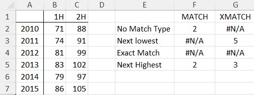
The following examples all lookup 80 in the range B2:B7
With no match type, MATCH defaults to next highest. However, MATCH produces nonsense results if the series are not ordered.
XMATCH defaults to exact match without a match type and correctly shows N/A when looking for 80 in this series. The next lowest is 79, in the 5th row and the next highest is 81 in the 3rd row.
We can use INDEX and XMATCH to identify a specific cell as in this formula: =INDEX(B2:C7,XMATCH(2012,A2:A7),XMATCH(“2H”,B1:C1))
This finds the row for 2012 and the columnn for 2H. It then finds the value in the cell for 2012, 2H.